Attribute focusing techniques for m-way association rules and
meta-rule guided mining for association rules with m predicates in
the rule require that all aggregates with m dimensions be
materialized. These are called essential
aggregates. Since data mining calculations are performed on the cubes
with at most m dimensions, the complete data cube is not
needed. Only cubes up to level m in the data cube lattice are
needed. To calculate this partial cube efficiently, a schedule is
required to minimize the intermediate calculations. Since the number
of aggregates is a fraction of the total number (![]() ) in a complete cube,
a different schedule, with additional optimizations to the ones discussed earlier,
is needed to minimize and calculate the intermediate,
non-essential aggregate calculations, that will help materialize the
essential aggregates.
) in a complete cube,
a different schedule, with additional optimizations to the ones discussed earlier,
is needed to minimize and calculate the intermediate,
non-essential aggregate calculations, that will help materialize the
essential aggregates.
Also, for a large number of dimensions it is impractical to calculate the complete data cube for OLAP. A subset of the aggregates can be materialized in our framework, and queries can be answered from the existing materializations, or some others can be calculated on the fly. Data cube reductions for OLAP have been topics of considerable research. [HRU96] has presented a greedy strategy to materialize the cubes depending on their benefit.
Consider a n dimensional data set and the cube lattice
discussed earlier and a level by level construction of the partial
data cube. The set of intermediate cubes between levels n and m
are essential if they are capable of calculating the next level
of essential cubes by aggregating a single dimension. This provides
the minimum set at a level k+1 which can cover the calculations at
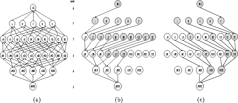
level k. To obtain the essential aggregates, we traverse the lattice
(Figure 3(a)), level by level starting from level 0. For a
level k, each entry has to be matched with the an entry from level
k+1, such that the cost of calculation is the lowest and the minimum
number of non-essential aggregates are calculated. We have to
determine the lowest number of non-essential intermediate aggregates
to be materialized. This can be done in one of two ways. For each
entry in level k we choose an arc to the leftmost entry in level
k+1, which it can be calculated from. This is referred to as the
left schedule shown in Figure 3(b). For example,
ABC has arcs to ABCD and ABCE, and the left schedule will choose
ABCD to calculate ABC. Similarly, a right schedule can be
calculated by considering the arcs from the right side of the lattice
(Figure 3(c)). Further optimizations on the left schedule
can be performed by replacing ![]() by
by ![]() , since ACE is also being materialized and the latter
involves a local calculation, if 2D partitioning is considered.
Of course, there are different trade-offs involved in choosing one over the
other, in terms of sizes of the cubes, partitioning of data on processors
and the inter-processor communication involved.
, since ACE is also being materialized and the latter
involves a local calculation, if 2D partitioning is considered.
Of course, there are different trade-offs involved in choosing one over the
other, in terms of sizes of the cubes, partitioning of data on processors
and the inter-processor communication involved.

Figure 3: (a) Lattice for cube operator (b) DAG for partial data cube (left schedule)
(c) right schedule